NVIDIA 2D Image and Signal Performance Primitives (NPP)

Based on the lack of examples and discussion in the forums, I assume the NPP are under-utilized and under-appreciated. Since I discovered these, it has been a game changer for me in my image processing work. Since machine vision camera resolutions are now at 12 Mega-pixels and higher, its required to accelerate processing with a GPU. No longer do I need to create many of my own Cuda algorithms for 2D image processing – many of them already exist.

For example, resizing an image (x,y re-scale) is fully supported on any pixel data type and with multiple filter types, all accelerated with Cuda parallel operations (see my post and example project on an image resize implementation here).

The NVIDIA documentation is a bit sparse, the shear number of functions and sub-libraries are daunting. I suggest starting with this page.

https://docs.nvidia.com/cuda/npp/modules.html

Within this page, open the topics and drill down, I think you will be impressed with the number of Cuda functions available.

May 23, 2023 Posted by admin | Cuda, Image Processing, NVIDIA Jetson | Comments Off on NVIDIA 2D Image and Signal Performance Primitives (NPP)

Calling Cuda functions from C#

This is a demonstration of creating a C# wrapper for a Cuda function.

The example Cuda function is ‘invertImageCuda()’ and it is contained in a Cuda dll called ‘image_processor.dll’. This dll file must exist in the same directory as the C# exe or in the path.

The C# File

In a C# file, create a C# entry point called ‘Invert()’. This entry point is a standard C# function and can be passed in any complex C# object type.

    /// <summary>
    /// Takes an array of float values, assumed to be pixels ranging from 0,1. Applies 'pixel = 1 - pixel' to all pixels in parallel Cuda operations.
    /// Original array is un-changed, inverted image is returned in a new array. 
    /// </summary>
    /// <param name="SrcPixels"></param>
    /// <param name="srcWidth"></param>
    /// <param name="srcHeight"></param>
    /// <returns></returns>
    public static float[] Invert(float[] SrcPixels, int srcWidth, int srcHeight)
    {
        float[] DstPixels = new float[srcWidth * srcHeight];

        unsafe
        {
            GCHandle handleSrcImage = GCHandle.Alloc(SrcPixels, GCHandleType.Pinned);
            float* srcPtr = (float*)handleSrcImage.AddrOfPinnedObject();

            GCHandle handleDstImage = GCHandle.Alloc(DstPixels, GCHandleType.Pinned);
            float* dstPtr = (float*)handleDstImage.AddrOfPinnedObject();

       
            // call a local function that takes c style raw pointers
            // this local function will in turn call the Cuda function
            invert(srcPtr, dstPtr, srcWidth, srcHeight);

            handleSrcImage.Free();
            handleDstImage.Free();
            GC.Collect();
        }
        return DstPixels;
    }

The ‘unsafe’ block tells C# that we are intentionally using raw c-style pointers. In the Visual Studio project properties editor, we must also check the box that allows un-safe code.

The GCHandle.Alloc() call creates a pinned pointer to a float[] so that the garbage collector cannot move the memory while the Cuda program is accessing it. We need to create a pinned pointer (GCHandle) for both the source and destination arrays.

The AddrOfPinnedObject() returns the pinned pointer that was allocated in the Alloc() function. We need c-style raw pointers to pass into the Cuda program.

A local function, invert(), will be called passing in only simple objects of pointers and int-s.

In the same C# file, create the Cuda wrapper function:

        [DllImport("image_processor.dll")]
        unsafe static extern int invertImageCuda(float* src, float* dst, Int32 width, Int32 sheight); 
        unsafe static int invert(float* src, float* dst, Int32 width, Int32 height)
        {
            return invertImageCuda(src, dst, width, height);
        }

The DllImport() line must be immediately above the Cuda function extern declaration and tells the compiler to look for invertImageCuda() in the dll.

The ‘invert()’ function is a local static, unsafe, function that accepts raw c-style pointers and then calls into the Cuda function, returning the value returned from Cuda (which is a success/error int value). The dst pointer is used by the Cuda function as the location to write the output values.

The Cuda File

In a separate Cuda file, in Cuda dll project, create the entry point:

//invertimage.h
#ifndef INVERTIMAGE_H
#define INVERTIMAGE_H
#include "cuda_runtime.h"
#include "device_launch_parameters.h"

// public


#ifdef __cplusplus
extern "C" {
#endif

#define CUDA_CLIB_EXPORTS
#ifdef CUDA_CLIB_EXPORTS
#define CUDA_CLIB_API __declspec(dllexport) 
#else
#define CUDA_CLIB_API __declspec(dllimport) 
#endif

    CUDA_CLIB_API cudaError_t invertImageCuda(float* src, float* dst, unsigned int width, unsigned int height);

#ifdef __cplusplus
}
#endif

//private

__global__ void invertImageKernel(float* src, float* dst, unsigned int width, unsigned int height);



#endif

This c header will not be read or used by the C# program, but rather, the C# compiler will rely on the invertImageCuda() matching declaration in the C# file. But this header with the CUDA_CLIB_API __declspec(dllexport) will tell the Cuda build to export this function as a public function. The CUDA_CLIB_EXPORTS preprocessor variable is defined locally because the cuda compiler of invert.cu will be the only compiler to see this code.

May 23, 2023 Posted by admin | Cuda | Comments Off on Calling Cuda functions from C#

create tensorflow data set from a list of numpy images

It took me a while to figure out the most optimal way to do this, so I thought I would share it.

I was originally using tf.stack() to create a tensor from a python list of numpy images. This operation was taking 3.37 seconds to stack a list of 40 images of 256x256x3 of type uint8.

Then I found tf.convert_to_tensor() and this reduced the operation down to 7 milliseconds.

    for image_file in images_list:
        img = cv2.imread(image_file)
        height,width= img.shape[:2]

        # my model design is based on creating 256x256 patches from larger images
        patches = patch_processor.extract_patches(img)


        tensor_list=[]
        for patch in patches:
            # convert 8 bit RGB image to floating point 0,1
            np_image_data = np.asarray(patch,dtype=np.float32)
            np_image_data = np_image_data / 127.5 - 1
            rgb_tensor = tf.convert_to_tensor(np_image_data, dtype=tf.float32)
            tensor_list.append(np.expand_dims(rgb_tensor, axis=0))
        
        # make one multi-demisional tensor that contains all the tensor patches for batch prediction


        ## this was taking 3.37 seconds for 36 images of 256x256
        #patches_tensor = tf.stack(tensor_list) 

        # convert python list to np array of image patches

        patches_tensor = np.array(tensor_list) 

        # create a tensorflow dataset from the array of image patches
        
        dataset1 = tf.data.Dataset.from_tensor_slices(patches_tensor) 
 
        # predict the patches

        predictions = model.predict( dataset1)

May 21, 2023 Posted by admin | Image Processing, Numpy, tensorflow | Comments Off on create tensorflow data set from a list of numpy images

Example implementation of nppiResize_32f_C1R_Ctx()

Project Source Code

The project source can be found here:

https://github.com/daviddrell/image_proc_samples

The project structure is Visual Studio 2019 with Cuda 11.7 installed. If you are using a different version of Cuda, I find the easiest was to solve this is to edit the Visual Studio project file in a text editor and change the version number there.

Overview

This is an example of re-scaling the size of the image in gray-scale floating point format accelerated using cuda on a GPU.

This example creates a simulated image of 2048×2048. In actual image processing applications you will have an image that comes from a jpeg or tiff file and must be decoded, often into an array of RGB bytes or directly into a gray-scale format. Many image processing operations occur on a gray-scale version of the image encoded as floating point, typically of values 0 to 1, or -1 to +1.

NVIDIA cuda comes with a library of basic image processing functions which are accelerated with parallel operations on the GPU, that run on top of the cuda library.

One of these functions is nppiResize_32f_C1R_Ctx(). The file resize.cpp implements all the memory operations necessary to resize an image using nppiResize_32f_C1R_Ctx().

The file resize.h provides a simple entry point for an image resize function which can be called from a c program with no knowledge of cuda programming.

Code Details

Refer to the gitlab project link. The sample entry point from a c programing perspective is given in main.cu. The example implementation of nppiResize_32f_C1R_Ctx() is given in resize.cpp.

Sample Results

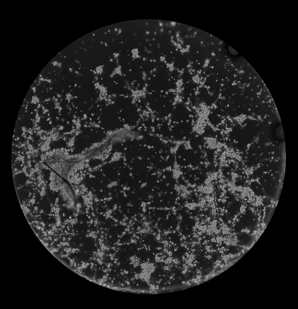
In a machine learning application, I needed to analyze a biological image (cells growing into vessel structures imaged under a microscope). The scientist provided images that were sized at 5995 x 6207 pixels. This size is too extreme for the requirements of extracting the structures. Additionally, the AI models were trained on images typically in the range of 1000×1000 to 2000×2000 pixels. So I scale down the images using the resize_Cuda() function demonstrated in the example project.

Here is the original image that is too large:

Here is the downsized image at 2000 x 2070 (the width was set to be 2000, our max AI trained size, the height was calculated to be 2070 to maintain the aspect ratio):

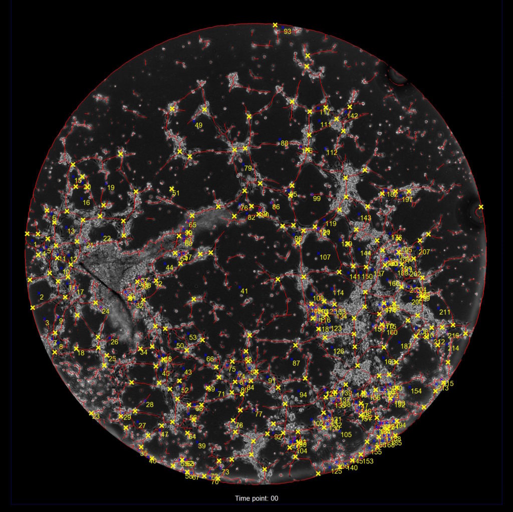
Here is the result of the analysis showing the branches and loops detected:

March 23, 2023 Posted by admin | Cuda | Cuda | Comments Off on Example implementation of nppiResize_32f_C1R_Ctx()

Save Framos IMX 253 images as Jpeg on NVIDIA Jetson

I was recently working on a demonstration of a Framos IMX 253 mono-chrome camera with a 12-bit sensor supported on a Jetson Xavier. For the demo, I needed to save the images as jpeg format. I thought it may be useful for others to see the inner-workings of a jpeg compression implementation Jetson, using the hardware assisted jpeg compressor.

The image came from the camera driver as 12 bit format in 16 bit integer array format. The sensor is mono-chrome, but the Jetson jpeg compressor only takes a single YUV format as input.

For this demo, I skip the step of re-mapping the luminance values from a 12 bit range to an 8 bit range and simply take the lower 8-bits. A production implementation needs a scheme for this re-mapping of luminance range. The implementation on a Jetson should take advantage of the hardware assist.

Step 1: get things setup


// Info is a structure provided from the caller that contains info about the frame 

// prepare to time execution of the jpeg compression    
auto start = std::chrono::steady_clock::now();

// prepare the output file
std::string outFile="/path/to/file.jpg";
std::ofstream* outFileStr = new std::ofstream(outFile);
if(!outFileStr->is_open())
        return false;

// create an instance of the nvidia jetson jpeg encoder

NvJPEGEncoder* jpegenc = NvJPEGEncoder::createJPEGEncoder("jpenenc");

// the jpeg output buffer size is 1.5 times the width*height 
unsigned long out_buf_size = Info.Width * Info.Height * 3 / 2;
unsigned char *out_buf = new unsigned char[out_buf_size];

Step 2: create an nvidia native buffer

// V4L2_PIX_FMT_YUV420M =  is the only format which appears to be supported by the Jetson jpeg encoder

// allocate the buffer    
NvBuffer buffer(V4L2_PIX_FMT_YUV420M, Info.Width, Info.Height , 0);

buffer.allocateMemory();

NvBuffer::NvBufferPlane* plane = &buffer.planes[0];

//convert the image luminance from uint16 to 8 bits and copy into the nvidia buffer
for(int y=0; y < Info.Height;y++)
{
    for(int x=0; x < Info.Width;x++)
    {
        plane->data[x+(y*plane->fmt.stride)] = (unsigned char) (m_img[x+(y*Info.Width)]);
    }
}

plane->bytesused = 1 * plane->fmt.stride * plane->fmt.height;

Step 3: the Framos camera driver provides a mono-chrome image, so make the image actually mono-chrome by setting the UV vectors to neutral color (127d).

 // initialize the Cb plan to the 127d value which means 0 color

plane = &buffer.planes[1];
char* data = (char *) plane->data;
plane->bytesused = 0;
for (int j = 0; j < plane->fmt.height; j++)
{
    memset(data,127,plane->fmt.width);
    data += plane->fmt.stride;
}
plane->bytesused = plane->fmt.stride * plane->fmt.height;

// initialize the Cr plan to the 127d value which means 0 color

plane = &buffer.planes[2];
data = (char *) plane->data;
plane->bytesused = 0;
for (int j = 0; j < plane->fmt.height; j++)
{
    memset(data,127,plane->fmt.width);
    data += plane->fmt.stride;
}
plane->bytesused = plane->fmt.stride * plane->fmt.height;

Step 4: run the actual jpeg encode function, save the file, and measure the results:

jpegenc->encodeFromBuffer(buffer, JCS_YCbCr, &out_buf, out_buf_size, 95);

auto end = std::chrono::steady_clock::now();

outFileStr->write((char *) out_buf, out_buf_size);
outFileStr->close();

printf( "Jpeg Encode Elapsed time in nanoseconds: %d\n",std::chrono::duration_cast<std::chrono::nanoseconds>(end - start).count());

delete[] out_buf;
delete outFileStr;

Result:

I am seeing roughly 25 milliseconds for the encode and save on an image 3840 x 2160 pixels.

March 20, 2023 Posted by admin | NVIDIA Jetson | Comments Off on Save Framos IMX 253 images as Jpeg on NVIDIA Jetson

Fun numpy things

Diff two images

diff_image = abs(prediction_mask - true_mask)

Count pixels that exactly match between two images

diff_image = abs(prediction_mask - true_mask)
matches = 1.0 * (diff_image == 0)
matches_count = np.sum(matches)

Count prediction pixels that do not match truth-mask pixels

diff_image = abs(prediction_mask - true_mask)
unpaired_pred_msk  = 1.0 * (prediction_mask>0) * (diff_img>0)       
un_matched_pred_count = np.sum(unpaired_pred_msk)

January 23, 2022 Posted by admin | Numpy | Comments Off on Fun numpy things

So what is numpy Matrix Multiplication?

What is the product of two matrices?

What is the dot product of two matrices?

What is the multiplication of two matrices?

I studied linear algebra in collage in 1984. I wrote my first computer program in Fortran in 1982 using punch cards. I wrote my first matrix multiplication program on an Texas Instruments Calculator in 1985. I started working with numpy matrices in 2019, which is 36 computer-age-years later.

At my first attempt at numpy matrix multiplication I did not get the expected results. As I dug into the documenation, I was very confused because the use of the words “multiply” and “matrix” have different meanings between my text book from late 20th century and early 21st century numpy.

Since I have not studied mathematics formally since completing my masters in the 1990s, I will not claim the linear algebra definitions have not changed, I will only refer to the “text book” I used in the 1980s.

Here is what I learned: numpy matrix multiplication is not mathematical matrix multiplication. But the numpy dot product is what I learned as matrix multiplication back in 1984, sort of….

Text book definition

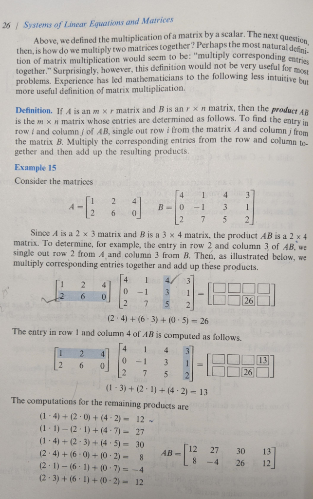
Here is my text book definition of the “product” of two matrices.

Elementary Linear Algebra, Fourth Edition, by Howard Anton

Notice the introduction to the concept at the top of the page, I quote:

Perhaps the most natural definition of matrix multiplication would seem to be: “multiply corresponding entries together.” Surprisingly, however, this definition would not be very useful for most problems.
P 26, Elementary Linear Algebra, Fourth Edition, by Howard Anton

The author explicitly says multiplying corresponding elements is not the definition of matrix multiplication, but this is precisely the numpy definition of matrix multiplication.

However, numpy does provide a mathematically correct method to compute the product of two matrices, referred to as the ‘dot’ product. To confuse matters more, in my text book, dot product refers only to vectors (1D matrices). In numpy, it refers to N-D matrices.

Definition of numpy Matrix Multiplication

For reference:

https://numpy.org/doc/stable/user/basics.broadcasting.html

https://numpy.org/doc/stable/reference/generated/numpy.multiply.html

The numpy.multiply() function simply multiplies corresponding elements. This requires that arrays have the same dimensions. If you attempt to multiply two matrices of different dimensions, numpy will either ‘broadcast’ the array to create a matching size, or throw an error if broadcasting will not work. For example:

Given $w = \begin{bmatrix} 1 & 5 & -3 & 2 \end{bmatrix}^T$ and $x=\begin{bmatrix} 8 & 2 & 4 & 7\end{bmatrix} ^T$

What is $w^T x?$

numpy array math is not standard mathmatics. As a python numpy developer you have to be very aware of the nuances of lists of numbers, lists of lists, numpy vectors and numpy arrays as the results you get on common operations will differ.

In this example I will only discuss the case of mumpy matrices (array with two dimensions). So, in python, using standard multiplication (* == np.multiply()):

>>> import numpy as np
>>> w = np.array([[1,5,-3,2] ]).transpose()    # defined as a numpy 2-D array of 1 x 4, if we used vectors, 
>>> x = np.array([ [8,2,4,7] ]).transpose()    #  the transpose would not work
>>> wt = w.transpose()
>>> wtx = wt * x
>>> wtx
array([[  8,  40, -24,  16],
       [  2,  10,  -6,   4],
       [  4,  20, -12,   8],
       [  7,  35, -21,  14]])

Notice we get a 4 x 4 matrix as a result. Not at all what we expect from the text book definition. The text book definition of multiplying a 1 x 4 vector with a 4 x 1 vector is a 1 dimensional entity, a scalar (in the example, the result should be the value of 20).

What happened was numpy first broad cast the arrays to match dimensions:

$wt = \begin{bmatrix} 1 & 5 & -3 & 2 \end{bmatrix}$ becomes:

$\begin{bmatrix} 1 & 5 & -3 & 2 \\ 1 & 5 & -3 & 2 \\ 1 & 5 & -3 & 2 \\ 1 & 5 & -3 & 2 \\ \end{bmatrix}$

and,

$x = \begin{bmatrix} 8 \\ 2 \\ 4 \\ 7 \end{bmatrix}$ becomes:

$\begin{bmatrix}8 & 8 & 8 & 8 \\2 & 2 & 2 & 2 \\4 & 4 & 4 & 4 \\7 & 7 & 7 & 7 \\\end{bmatrix}$

So simply multiplying the corresponding elements we get a 4 x 4 matrix:

$\begin{bmatrix}8 & 40 & -24 & 16 \\2 & 10 & -6 & 4 \\4 & 20 & -12 & 8 \\7 & 35 & -21 & 14 \\\end{bmatrix}$

Getting the Mathematically Correct Answer

To get the text book correct result, just use the numpy dot() method:

>>> wtx = wt.dot(x)
>>> wtx
array([[20]])

But be aware, the correct format of the answer should be the scaler value 20, which numpy displays a 1 x 1 matrix.

October 9, 2021 Posted by admin | Numpy | Comments Off on So what is numpy Matrix Multiplication?

Numpy Dot Product of Vectors

Mathematical Definition of a Dot Product

The dot product of two vectors $\vec{A} = (a_1, a_2, a_3)$ and $\vec{B} = (b_1, b_2, b_3)$ is a scaler given by:

$\vec{A}\cdot \vec{B}= a_1 b_1 + a_2 b_2 + a_3 b_3$

Vectors In Python/Numpy

How can we use numpy to solve generalized vector dot products such as the one below:

Given $a = \begin{bmatrix} 1 & 5 & -3 & 2 \end{bmatrix}^T$ and $b=\begin{bmatrix} 8 & 2 & 4 & 7\end{bmatrix} ^T$

What is $a^T b?$

Using python and the numpy library, we have two options for expressing this calculation, 1-D arrays, and matrices. But each has a caveat to consider.

In all code examples below assume we have imported the numpy library:


>>> import numpy as np

Vector as 1-D Array

In python, using the numpy library, a vector can be represented as 1-D array or an Nx1 (or 1xN) matrix. For example:

>>> a = np.array([1,5,-3,2])       # create 1-D array, a simple list of numbers
>>> a
array([ 1,  5, -3,  2])
>>> a.shape
(4,)                               # shape is shown to be a 1-D array

If we take a transpose of the 1-D array, numpy will return the same dimension. So a transpose function has no effect on a numpy 1-D array.

>>> a
array([ 1,  5, -3,  2])
>>> a.shape               # shape of a is 4
(4,)
>>> at = a.transpose()

>>> at.shape
(4,)
>>> at
array([ 1,  5, -3,  2])  # shape of a-transpose is also 4

>>> at.shape
(4,)

So if we define a vector ‘a’ and a vector ‘b’ and try to find the dot product of the transpose of ‘a’ to ‘b’, the transpose will have no effect, but numpy will dot product the two single dimension vectors with this result:

>>> a
array([ 1,  5, -3,  2])
>>> b
array([8, 2, 4, 7])

>>> c = np.dot(a,b)   # take the dot product of 1-D vectors a and b
>>> c
20                     # the result is a scalar of value 20

Note the result is the expected value of 20, and it is a scalar as expected. So when using numpy 1-D arrays for dot products, the user has to be aware that transpose functions are meaningless but also will not affect the dot product result.

Vector as a row/column of a 2-D Matrix

If we create the vector a as a numpy 2-D matrix by using the double brackets (single row, multi-column), the resulting matrix is shown below.

>>> a = np.array([ [1,5,-3,2]  ])   # single row, multi-column array with dimensions 1x4
>>> a
array([[ 1,  5, -3,  2]])
>>> a.shape
(1, 4)                              # shape is shown to be a NxM array with N=1, M=4

If we then take the transpose of a, we get:

>>> at = a.transpose()
>>> at                   # the transpose of a is now a 4x1 (4 row, 1 col) matrix
array([[ 1],
       [ 5],
       [-3],
       [ 2]])
>>> at.shape
(4, 1)                   # shape is shown to be a NxM array with N=4, M=1

So back to our generalized problem (defined above), what is $a^T b?$ , using numpy matrices:

a = np.array([ [1,5,-3,2]  ]).transpose()  # implement a as given above
at = a.transpose()                        # get a transpose
b = np.array([ [8,2,4,7]  ]).transpose()   # implement b as given above
c = np.dot(at,b)                           # get the aT dot b 
>>> c                                      # print the contents of c
array([[20]])

We see that we can use the transpose as expected, and get the expected result of 20, but the result is expressed as a 1×1 matrix rather than the expected scaler.

Also, note, dot products of matrices are only defined as the product of matrices with orthogonal dimensions of (1xN dot Nx1), or (Nx1 dot 1xN). If you attempt to take the dot product of a Nx1 and Nx1, for example, you will get an error:

>>> c=np.dot(a,b)
Traceback (most recent call last):
  File "<stdin>", line 1, in <module>
  File "<__array_function__ internals>", line 6, in dot
ValueError: shapes (1,4) and (1,4) not aligned: 4 (dim 1) != 1 (dim 0)

Conclusion

If numpy 1-D arrays are used for dot product, the user has to understand that transpose functions have no meaning. On the other hand, if numpy matrices are used, the transpose function has the expected meaning but the user has to remember to translate the 1×1 matrix result to a scaler result.

September 19, 2021 Posted by admin | Numpy | Comments Off on Numpy Dot Product of Vectors

David W Drell